MNIST Anomaly Detection

Baseline from: https://arxiv.org/pdf/2006.02516.pdf

• 14x14, [\(0-1\)] range, pixels flattened (dont exploit inherent locality)

• Embedding: TrigonometricEmbedding (p=2)

• Combined loss: \(\mathcal{L} = \frac{1}{N}\sum_{i=1}^{N} \left( \log \left\| P \Phi({X_i}) \right\|_2^2 - 1 \right)^2 + \alpha \cdot \mathrm{ReLU}\left(\log(\|P\|_F^2)\right)\)

Imports

import os

os.environ["KMP_WARNINGS"] = "0"
import jax
import jax.numpy as jnp
import matplotlib.pyplot as plt
import numpy as np
import optax
import tensorflow as tf
from jax.nn.initializers import *
from sklearn.metrics import auc
from tensorflow.keras.datasets import mnist

from tn4ml.embeddings import *
from tn4ml.eval import *
from tn4ml.initializers import *
from tn4ml.metrics import *
from tn4ml.models.model import *
from tn4ml.models.smpo import *
from tn4ml.util import *

jax.config.update("jax_enable_x64", True)

Load dataset

train, test = mnist.load_data()
data = {
    "X": {"train": train[0], "test": test[0]},
    "y": {"train": train[1], "test": test[1]},
}

normal_class = 0

X = {
    "normal": data["X"]["train"][data["y"]["train"] == normal_class] / 255.0,
    "anomaly": data["X"]["train"][data["y"]["train"] != normal_class] / 255.0,
}

X_test = {
    "normal": data["X"]["test"][data["y"]["test"] == normal_class] / 255.0,
    "anomaly": data["X"]["test"][data["y"]["test"] != normal_class] / 255.0,
}

# Function to resize images to 14x14
def resize_images(images):
    """Resize a batch of images to 14x14 pixels."""
    resized_images = tf.image.resize(
        images, [14, 14], method=tf.image.ResizeMethod.AREA
    )
    return resized_images.numpy()

X_resized = {
    "normal": resize_images(np.expand_dims(X["normal"], axis=-1)),
    "anomaly": resize_images(np.expand_dims(X["anomaly"], axis=-1)),
}

X_test_resized = {
    "normal": resize_images(np.expand_dims(X_test["normal"], axis=-1)),
    "anomaly": resize_images(np.expand_dims(X_test["anomaly"], axis=-1)),
}

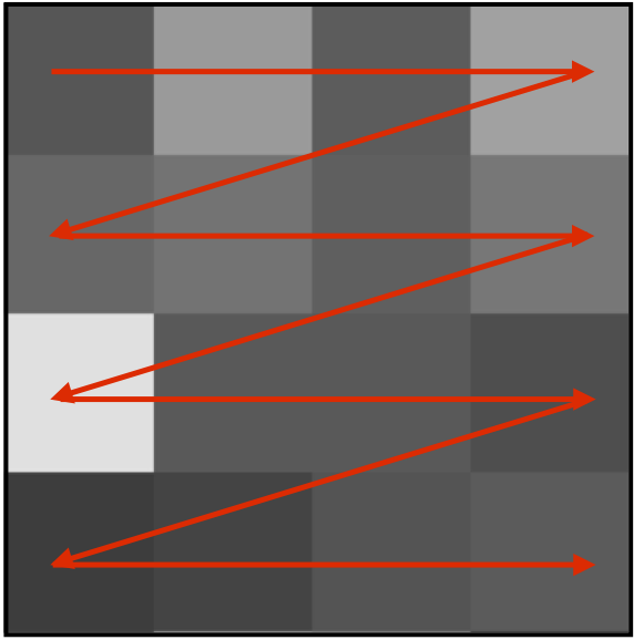
Rearrange pixels in zig-zag order

• (from https://arxiv.org/pdf/1605.05775.pdf)

def zigzag_order(data):
    """Flatten image rows into a zigzag-compatible feature order."""
    data = np.squeeze(data)
    data_zigzag = []
    for x in data:
        image = []
        for i in x:
            image.extend(i)
        data_zigzag.append(image)
    return np.asarray(data_zigzag)

zigzag = True

if zigzag:
    train_normal = zigzag_order(X_resized["normal"])
    test_normal = zigzag_order(X_test_resized["normal"])

    train_anomaly = zigzag_order(X_resized["anomaly"])
    test_anomaly = zigzag_order(X_test_resized["anomaly"])
else:
    train_normal = X_resized["normal"].reshape(
        -1, X_resized["normal"].shape[1] * X_resized["normal"].shape[2]
    )
    test_normal = X_test_resized["normal"].reshape(
        -1, X_test_resized["normal"].shape[1] * X_test_resized["normal"].shape[2]
    )

    train_anomaly = X_resized["anomaly"].reshape(
        -1, X_resized["anomaly"].shape[1] * X_resized["anomaly"].shape[2]
    )
    test_anomaly = X_test_resized["anomaly"].reshape(
        -1, X_test_resized["anomaly"].shape[1] * X_test_resized["anomaly"].shape[2]
    )

Training setup

L = 196
initializer = gramschmidt("normal", 1e-1)
key = jax.random.key(42)
shape_method = "noteven"
bond_dim = 10
phys_dim = (2, 2)
spacing = 8
add_identity = True
boundary = "obc"

model = SMPO_initialize(
    L=L,
    initializer=initializer,
    key=key,
    shape_method=shape_method,
    spacing=spacing,
    bond_dim=bond_dim,
    phys_dim=phys_dim,
    cyclic=False,
    compress=True,
    add_identity=add_identity,
    boundary=boundary,
)

alpha = 0.4


def loss_combined(*args, **kwargs):
    """Compute the combined reconstruction and regularization loss."""
    error = LogQuadNorm
    reg = LogReLUFrobNorm
    return CombinedLoss(*args, **kwargs, error=error, reg=lambda P: alpha * reg(P))

Define training parameters

epochs = 100
batch_size = 512
optimizer = optax.adam
strategy = "global"
loss = loss_combined
train_type = TrainingType.UNSUPERVISED
embedding = TrigonometricEmbedding()
learning_rate = 1e-3
earlystop = EarlyStopping(min_delta=0, patience=5, monitor="loss", mode="min")

model.configure(
    optimizer=optimizer,
    strategy=strategy,
    loss=loss,
    train_type=train_type,
    learning_rate=learning_rate,
)

history = model.train(
    train_normal,
    epochs=epochs,
    batch_size=batch_size,
    embedding=embedding,
    normalize=True,
    earlystop=earlystop,
    dtype=jnp.float64,
)

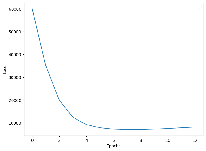
epoch:   8%|▊          8/100 , loss=7000.6899

Waiting for 1 epochs.

epoch:   9%|▉          9/100 , loss=7024.4809

Waiting for 2 epochs.

epoch:  10%|█          10/100 , loss=7226.5291

Waiting for 3 epochs.

epoch:  11%|█          11/100 , loss=7517.7869

Waiting for 4 epochs.

epoch:  12%|█▏         12/100 , loss=7839.7346

Training stopped by EarlyStopping on epoch: 7

epoch:  13%|█▎         13/100 , loss=8161.6364

plot_loss(history, validation=False, figsize=(8, 6))

Evaluate

indices = list(range(len(test_anomaly)))
rng = np.random.default_rng()
rng.shuffle(indices)

indices = indices[: len(test_normal)]
test_anomaly = np.take(test_anomaly, indices, axis=0)

loss = LogQuadNorm

anomaly_score = model.evaluate(
    test_anomaly,
    evaluate_type=train_type,
    return_list=True,
    dtype=jnp.float64,
    batch_size=128,
    embedding=embedding,
    metric=loss,
)
normal_score = model.evaluate(
    test_normal,
    evaluate_type=train_type,
    return_list=True,
    dtype=jnp.float64,
    batch_size=128,
    embedding=embedding,
    metric=loss,
)

Plot anomaly scores and ROC curve

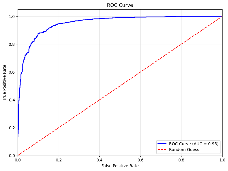
fpr, tpr = get_roc_curve_data(normal_score, anomaly_score, anomaly_det=True)
auc_value = auc(fpr, tpr)

plt.figure()
plt.hist(anomaly_score, bins=100, histtype="step", label="anomaly", color="red")
plt.hist(normal_score, bins=100, histtype="step", label="normal", color="blue")
plt.title("Anomaly score distribution")
plt.legend()
plt.text(
    0.5, -0.1, f"AUC Value: {auc_value}", ha="center", transform=plt.gca().transAxes
)
plt.legend()
plt.show()

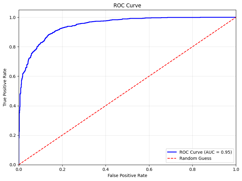
# Plot ROC curve
plot_ROC_curve_from_data(fpr, tpr)