MNIST classification

import os

os.environ["KMP_WARNINGS"] = "0"
import jax
import jax.numpy as jnp
import numpy as np
import tensorflow as tf
from jax.nn.initializers import *
from tensorflow.keras.datasets import mnist

from tn4ml.embeddings import *
from tn4ml.eval import *
from tn4ml.initializers import *
from tn4ml.metrics import *
from tn4ml.models.model import *
from tn4ml.models.mps import *
from tn4ml.strategy import *
from tn4ml.util import *

# Enable 64-bit precision and set matmul precision to highest

jax.config.update("jax_enable_x64", True)
jax.config.update("jax_default_matmul_precision", "highest")

Load dataset

MNIST images → grayscale images

• size: 28x28

• 0-9 numbers

train, test = mnist.load_data()

if os.environ.get("CI"):
    train = (train[0][:256], train[1][:256])
    test = (test[0][:64], test[1][:64])

train_labels = train[1]
train_images = train[0].reshape(-1, 28, 28)

import matplotlib.pyplot as plt

hfont = {"fontname": "Courier New", "fontsize": 15, "fontweight": "bold"}

for i in range(10):
    plt.subplot(2, 5, i + 1)
    # Select the first image of each digit
    digit_indices = np.where(train_labels == i)[0]
    plt.imshow(train_images[digit_indices[0]], cmap="gray")
    plt.title(f"Label: {i}", **hfont)
    plt.axis("off")

plt.tight_layout()

data = {
    "X": {"train": train[0], "test": test[0]},
    "y": {"train": train[1], "test": test[1]},
}

Reduce size of the image

def resize_images(images):
    """Resize a batch of images to 14x14 pixels."""
    resized_images = tf.image.resize(
        images, [14, 14], method=tf.image.ResizeMethod.AREA
    )
    return resized_images.numpy()

X_resized = (
    resize_images(data["X"]["train"].reshape(-1, 28, 28, 1)).reshape(-1, 14, 14) / 255.0
)

X_test_resized = (
    resize_images(data["X"]["test"].reshape(-1, 28, 28, 1)).reshape(-1, 14, 14) / 255.0
)

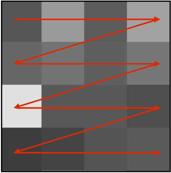
Rearagne pixels in zig-zag order

• ref. - Supervised learning with quantum-inspired tensor networks (https://arxiv.org/pdf/1605.05775.pdf)

def zigzag_order(data):
    """Flatten image rows into a zigzag-compatible feature order."""
    data_zigzag = []
    for x in data:
        image = []
        for i in x:
            image.extend(i)
        data_zigzag.append(image)
    return np.asarray(data_zigzag)

train_data = zigzag_order(X_resized)
test_data = zigzag_order(X_test_resized)

One-hot encoding of labels

10 classes: 0, 1, 2, 3, 4, 5, 6, 7, 8, 9

Label 0 → [1, 0, 0, 0, 0, 0, 0, 0, 0, 0] Label 1 → [0, 1, 0, 0, 0, 0, 0, 0, 0, 0] Label 2 → [0, 0, 1, 0, 0, 0, 0, 0, 0, 0] Label 3 → [0, 0, 0, 1, 0, 0, 0, 0, 0, 0] Label 4 → [0, 0, 0, 0, 1, 0, 0, 0, 0, 0] Label 5 → [0, 0, 0, 0, 0, 1, 0, 0, 0, 0] Label 6 → [0, 0, 0, 0, 0, 0, 1, 0, 0, 0] Label 7 → [0, 0, 0, 0, 0, 0, 0, 1, 0, 0] Label 8 → [0, 0, 0, 0, 0, 0, 0, 0, 1, 0] Label 9 → [0, 0, 0, 0, 0, 0, 0, 0, 0, 1]

n_classes = 10

y_train = integer_to_one_hot(data["y"]["train"], n_classes)
y_test = integer_to_one_hot(data["y"]["test"], n_classes)

Take samples for training, validation and testing

from sklearn.model_selection import train_test_split

train_inputs, _, train_targets, _ = train_test_split(
    train_data, y_train, test_size=0.8 if os.environ.get("CI") else 0.9, random_state=42
)  # take only part of the training data - to speed up the training

train_inputs, val_inputs, train_targets, val_targets = train_test_split(
    train_inputs, train_targets, test_size=0.2, random_state=42
)

TN as ML model

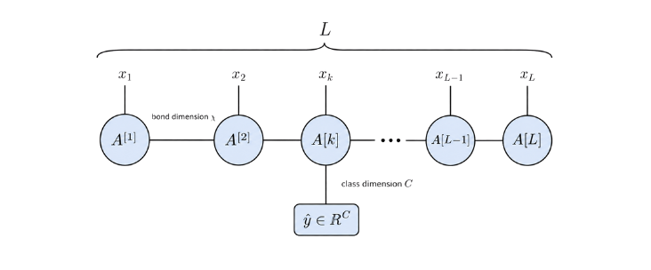
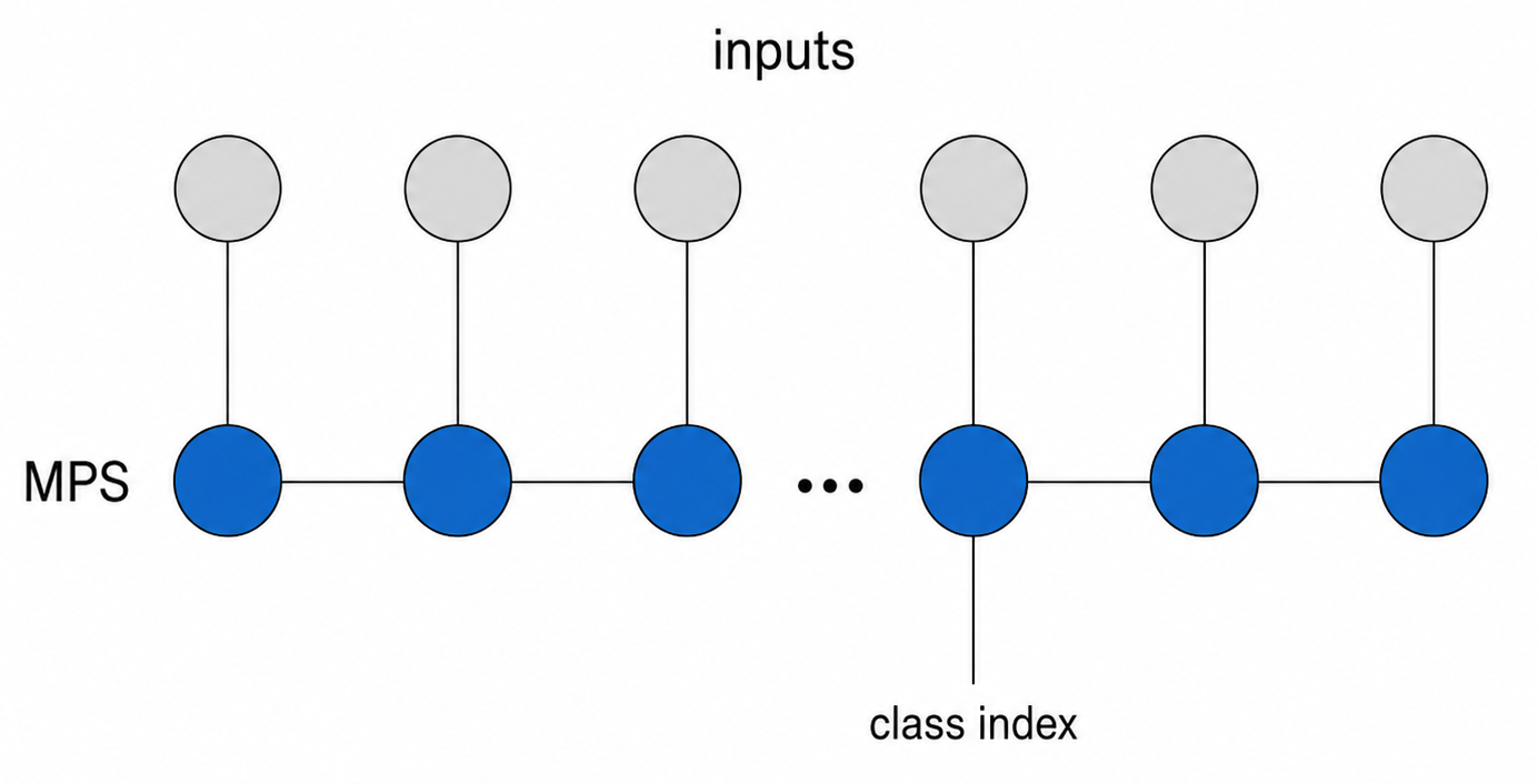
MPS-based classifier:

• each circular node represents a tensor (\(A^{[i]}\)) in the Matrix Product State chain

• vertical legs correspond to local input features (\(x_i\))

• horizontal connections represent contracted virtual bonds with bond dimension (\(\chi\))

• designated tensor carries an additional output leg of dimension (\(C\)), producing the class-score vector (\(\hat{y} \in \mathbb{R}^C\)) used for classification

Specify parameters and initialize a tensor network

L = 14 * 14  # number of tensors in the MPS
initializer = randn(1e-2)  # MPS tensors are initialized with random normal values
key = jax.random.key(42)
shape_method = "noteven"
bond_dim = 10  # bond dimension of the MPS
phys_dim = 3  # when polyomial embedding is used p = 3, when trigonometric embedding is used p = 2
class_dim = 10  # number of classes
index_class = L // 2 if L % 2 == 0 else L // 2 + 1
cyclic = False
add_identity = True
boundary = "obc"  # open boundary conditions

model = MPS_initialize(
    L,
    initializer=initializer,
    key=key,
    shape_method=shape_method,
    bond_dim=bond_dim,
    phys_dim=phys_dim,
    cyclic=False,
    add_identity=add_identity,
    class_dim=class_dim,
    class_index=index_class,
    canonical_center=index_class,
    boundary=boundary,
    dtype=jnp.float64,
)

Define training parameters

def cross_entropy_loss(*args, **kwargs):
    """Compute softmax cross-entropy loss."""
    return OptaxWrapper(optax.softmax_cross_entropy)(*args, **kwargs).mean()

# training parameters
optimizer = optax.adam
strategy = "global"  # Global Gradient Descent
loss = cross_entropy_loss
train_type = TrainingType.SUPERVISED
embedding = PolynomialEmbedding(degree=2, n=1, include_bias=True)  # if using randn
learning_rate = 1e-3
device = ("cpu", 0)

model.configure(
    optimizer=optimizer,
    strategy=strategy,
    loss=loss,
    train_type=train_type,
    learning_rate=learning_rate,
    device=device,
)

epochs = 1 if os.environ.get("CI") else 50
batch_size = 16 if os.environ.get("CI") else 1000

To obtain loss scalar value, contract:

history = model.train(
    train_inputs,
    targets=train_targets,
    val_inputs=val_inputs,
    val_targets=val_targets,
    epochs=epochs,
    batch_size=batch_size,
    canonize=(True, index_class),
    embedding=embedding,
    normalize=True,
    display_val_acc=True,
    val_batch_size=batch_size,
    eval_metric=cross_entropy_loss,
    dtype=jnp.float64,
)

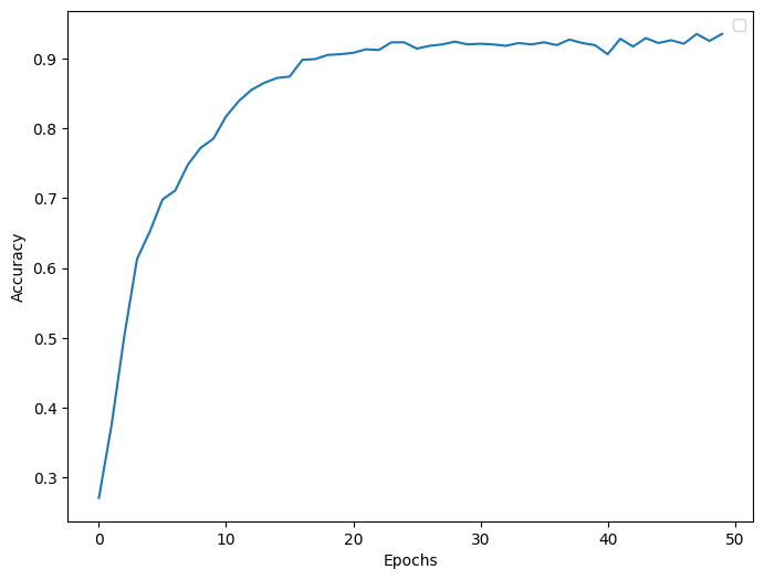
epoch: 100%|██████████ 50/50 , loss=1.4784, val_loss=1.5175, val_acc=0.9350

plot_loss(history, validation=True, figsize=(8, 6))

plot_accuracy(history, figsize=(8, 6))

Save model

model.save(
    "model", "/tmp", tn=True
)  # tn=True because MPS for classification if TensorNetwork object

Evaluate

Calculate accuracy of the classification

model.accuracy(
    test_data,
    y_test,
    embedding=embedding,
    batch_size=16 if os.environ.get("CI") else 512,
)

0.9369860197368421

Retrain with exponential decay

# Exponential decay of the learning rate.
scheduler = optax.exponential_decay(
    init_value=1e-3, transition_steps=1000, decay_rate=0.01
)

# Combining gradient transforms using `optax.chain`.
gradient_transforms = [
    optax.clip_by_global_norm(1.0),  # Clip by the gradient by the global norm.
    optax.scale_by_adam(),  # Use the updates from adam.
    optax.scale_by_schedule(scheduler),  # Use the learning rate from the scheduler.
    # Scale updates by -1 since optax.apply_updates is additive and we want to descend on the loss.
    optax.scale(-1.0),
]

model.configure(
    gradient_transforms=gradient_transforms,
    strategy=strategy,
    loss=loss,
    train_type=train_type,
    learning_rate=learning_rate,
)

epochs = 1 if os.environ.get("CI") else 50
batch_size = 16 if os.environ.get("CI") else 1000

history = model.train(
    train_inputs,
    targets=train_targets,
    val_inputs=val_inputs,
    val_targets=val_targets,
    epochs=epochs,
    batch_size=batch_size,
    canonize=(True, index_class),
    embedding=embedding,
    normalize=True,
    display_val_acc=True,
    eval_metric=cross_entropy_loss,
    val_batch_size=batch_size,
    dtype=jnp.float64,
)

epoch: 100%|██████████ 50/50 , loss=1.4502, val_loss=1.5027, val_acc=0.9360

model.accuracy(
    test_data,
    y_test,
    embedding=embedding,
    batch_size=16 if os.environ.get("CI") else 1000,
)

0.9459