Introduction to Tensor Networks

Tensor Networks (TNs) are renowned for their ability to approximate ground states in quantum physics. Over time, their application has expanded beyond quantum mechanics to a wide range of fields, particularly Machine Learning.

Overview

1. Basic operations with tensors

2. Contractions

3. Creation of Tensor Network

4. MNIST classification with MPS

import os

os.environ["KMP_WARNINGS"] = "0"

import jax
import numpy as np
import quimb.tensor as qtn
from jax.nn.initializers import *

from tn4ml.embeddings import *
from tn4ml.initializers import *
from tn4ml.metrics import *
from tn4ml.models.model import *
from tn4ml.models.mps import *
from tn4ml.strategy import *
from tn4ml.util import *

jax.config.update("jax_enable_x64", True)

Basic operations with tensors

The primary strength of Tensor Networks (TNs) lies in their ability to easily contract and split tensor indices. By taking a large tensor with many indices (a rank-L tensor), we can reconfigure it into a more convenient form. This reconfiguration allows us to apply advanced linear algebra tools that are typically only available for matrices.

From Vector to Matrix = Index Splitting

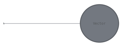
Imagine having a vector (rank-1 tensor) \(T_k\) where \(k=\underbrace{1,2,\dotsc,i-1,i}_{i},\underbrace{i+1,\dotsc,N}_{j}\). Then, we can see that

\[T_k = T_{i,j}\]

Now \(T\) is represented as a matrix.

data - raw data array inds - a set of ‘indices’ to label each dimension with tags - name of a tensor

# visualize a vector
data = np.array([1, 0, 0, 1])
inds = "k"
tags = ("Vector",)

ket = qtn.Tensor(data=data, inds=inds, tags=tags)
ket.draw()

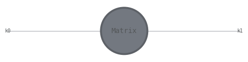
# visualize a matrix
data = data.reshape((2, 2))  # reshape vector to matrix
inds = ("k0", "k1")
tags = ("Matrix",)
ket = qtn.Tensor(data=data, inds=inds, tags=tags)
ket.draw()

Singular Value Decomposition

qtn.decomp.svdvals(ket.data)  # singular values of the matrix

array([1., 1.])

Contraction

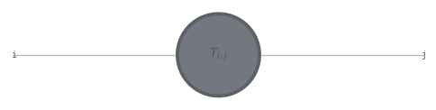
As we just demonstrated, it’s possible to reverse the splitting of tensor indices and fuse two (or more) indices together. By doing so, a rank-2 tensor (a matrix) \(T_{i,j}\) can be fused to form a single global index, allowing it to be contracted with another tensor \(A_k\).

data = np.array([[1, 0], [0, 1]])
ket = qtn.Tensor(data=data, inds=("i", "j"), tags=("$T_{i,j}$",))
ket.draw()

From Matrix to Vector = Index Fusion

T_k = ket.fuse({"k": ("i", "j")}).retag({"$T_{i,j}$": "$T_k$"})
T_k.draw()

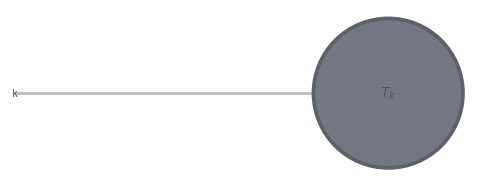
This contraction is feasible when the dimensions of the indices being contracted match. Specifically, the dimension of \(k\) must equal the combined dimension of \(ij\), such as \(dim(k) = dim(ij)\). Thus, the contraction is expressed as:

\[T_{i,j} A_k = T_k A_k = s\]

where s is a rank-\(0\) tensor, meaning that is a scalar.

A_k = qtn.Tensor(np.array([1, 1, 0, 0]), inds=("k"), tags=("$A_k$",))
s = A_k | T_k
s.draw()

Result of contraction vector-vector = scalar

s.contract()

1

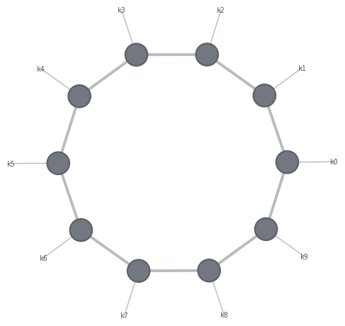
Create a Tensor Network

(example from Quimb)

1. Create list of tensors

2. Add physical indices to each tensor - Tensor.new_ind()

3. Add bonds between neighbouring tensors - Tensor.new_bond()

4. Create TensorNetwork object with these tensors

L = 10

# create the nodes, by default just the scalar 1.0
tensors = [qtn.Tensor() for _ in range(L)]

for i in range(L):
    # add the physical indices, each of size 2
    tensors[i].new_ind(f"k{i}", size=2)

    # add bonds between neighbouring tensors, of size 7
    tensors[i].new_bond(tensors[(i + 1) % L], size=7)

mps = qtn.TensorNetwork(tensors)
mps.draw()

Contraction of TN

Tensor network can be contracted to one tensor of rank \(N\), where \(N\) is number of tensors in TN.

tensor = mps ^ all
print(tensor)

Tensor(shape=(2, 2, 2, 2, 2, 2, 2, 2, 2, 2), inds=('k0', 'k1', 'k2', 'k3', 'k4', 'k5', 'k6', 'k7', 'k8', 'k9'), tags=oset([]), backend='numpy', dtype='float64')